In this article, you’ll learn the available ways to insert pictures/images to Excel cells, and how to customize the appearance of the inserted images.
While Microsoft Excel is primarily focused on working with numbers and text, there are situations where you may need to insert images or photos to make it easier to understand and analyze the data.
In previous versions of Excel, you could only place the image on the tope of the cell and adjust its properties to make it move and resize with the cells. But now, Excel has new features that let you to insert images right inside a cell. This means that images are treated like any other data type, such as text or numbers, and can be formatted according to your preference.
How to Insert an Image/Picture to an Excel Cell.
1. Add Images to Excel with “Insert Pictures” feature.
2. Insert Images/Pictures to Excel with Copy-Paste.
3. Import Online Images to Excel using the IMAGE function.
Method 1. Insert Picture in a Cell using the ‘Insert Pictures’ feature.
The usual method to insert a picture in an Excel cell is by using the “Insert > Pictures” option. The “Insert Pictures” feature allows you to import images into cells from your computer, the Microsoft’s stock image library (if you have an O365 account), or even images from the Internet.
To import a picture/image to an Excel worksheet:
1. Open the Excel worksheet where you want to insert the image.
2. Select the cell where you want the image to be inserted.


3. In the Excel ribbon, click the Insert tab and click on Pictures drop-down menu.


3a. In the drop-down menu that appears, choose one of the following options based on where the image that you want to import is located:
● This Device: To insert an image/picture stored on your local device.
● Stock Images: To insert a free image image/picture or icon provided by Microsoft library. (This option is only available only to Microsoft 365/Office 365 subscriptions)
● Online Pictures:To insert an Online Image (from the Internet).
![clip_image002[9]](https://techprotips.com/wp-content/uploads/2023/10/localimages/clip_image0029.png "clip_image002[9]")
![clip_image002[9]](https://techprotips.com/wp-content/uploads/2023/10/localimages/clip_image0029_thumb.png "clip_image002[9]")
This Device.
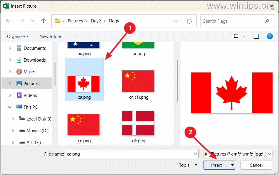
1. To insert an Image/Picture in Excel stored on your local computer, go to Insert > Pictures and click This Device.


2. Then, navigate to the location where the image is stored, select it and click Insert. *
* Note: To insert multiple images, hold the Ctrl key while selecting the images, then click on Insert.
From Stock images*
The Stock Images are provided by Microsoft for free and can be used to enhance the visual appeal in your Excel documents.
1. To insert an image in Excel from the free stock images, go to Insert > Pictures and click Stock Images.*
* Note: The “Stock Images” option is available only to Office365/Microsoft365 subscriptions.


2. Then browse through the available images and click on the one you want to insert into your spreadsheet. Then click Insert, to add the image into the selected cell.
* Notes:
1. To easily locate a desired image, search for it by describing it. (e.g. “Clouds in the Sky”).
2. The number of free stock images available is limited, and to access the entire catalog of stock images, you need to have a Microsoft 365 subscription.


From Online Pictures
In Microsoft Excel, the “Online Pictures” feature allows you to search for and insert images directly from online sources, such as your OneDrive or by using the Bing Image Search, into your Excel spreadsheets. *
* Note: If you want to insert an online image, using the image’s URL address, see the instructions on method-3 below.
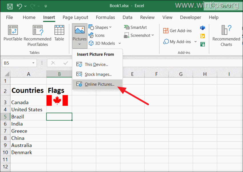
1. To insert an Online image, go to Insert > Pictures and click Online Pictures option.


2. In the “Online Pictures” dialog box that will appear, type in the search bar a keyword related to the image you want to insert and hit Enter.
3. After the images appear (optionally):
- Click the Creative Commons only button, if you want to display only the images that can be used without Copyright issues.
- Click the Filter icon

 to filter the images according to their Size, Type, Layout and Color.


4. Finally, select the image you want to add to your Excel worksheet and click on Insert button.
![clip_image016[6]](https://techprotips.com/wp-content/uploads/2023/10/localimages/clip_image0166.png "clip_image016[6]")
![clip_image016[6]](https://techprotips.com/wp-content/uploads/2023/10/localimages/clip_image0166_thumb.png "clip_image016[6]")
5. That’s it! The selected image will be inserted into the cell you initially selected. However, regardless of the option you choose, the inserted image will not automatically fit into the cell unless the image is relatively small in size.


How to Customize Image Size and Position in Excel.
As you can see above, when you insert an image, it will be inserted at its original size. If you want to resize the image to fit the cell, follow one the ways below:
Way 1. Resize the Image by dragging its edges.
1. Place your cursor over any corner or edge of the image until it changes to a double-headed arrow.
2. Then, click and drag the corner or edge of the image to resize it to match the size of the cell.


Way 2. Resize the Image by pressing the ALT key.
Another way to resize the inserted image in the cell, is to press and hold the the ALT key, while clicking and dragging the corner of the image. As you move the picture close to the border of the cell, it will automatically snap and align itself with the cell’s border.


How to Lock Image/Picture to Cell in Excel
When you insert a picture into an Excel cell, the image will not remain attached to the cell when you move or resize cells within the worksheet. If you want to lock it to ensure that it moves, resizes, filters, and hides along with the cell, do the following:
1. Right-click the picture you want to lock and select Format Picture from the context menu.


2. In the “Format Picture” pane that appears on the right side of the window, select the Size & Properties icon and then click the Properties option to expand it.


3. Then, select the Move and size with cells option to lock the picture with the cell.*
* Note: This option doesn’t mean the picture is stuck in one cell and can’t be moved. You can still move it to other cells. This means you’re free to move cells around, filter them, or hide them, and the picture will move, be filtered, or hide along with the cells.


Method 2. Insert Picture in Excel Cell with Copy-Paste.
Excel also provides the option to copy and paste images into cells from other programs. To paste a picture in Excel from another program, follow these simple steps:
1. Select the image you want to insert in the other program (such as Microsoft Paint, Word, or Adobe Photoshop).
2. Press Ctrl + C to copy the image.
3. Switch back to Excel and select the cell where you want to place the image.
4. Press Ctrl + V to paste the image.
5. After pasting the image, you can resize it to fit inside the cell, using the instructions above.


Method 3. Insert Picture in Excel Cell using the IMAGE function.
The third method to insert an image to Excel, is by using the “IMAGE” function. This method is useful when you want to insert an online image to Excel, by using the image’s URL.
The Image Function supports the following Image types: BMP, JPG/JPEG, GIF, TIFF, PNG, ICO, and WEBP.
However, it is important to know that the IMAGE function is only accessible in Microsoft 365 and Excel for the web.
To insert an picture in Excel using the IMAGE function, use this syntax: *
- =IMAGE(source, [alt_text], [sizing], [height], [width]),
* Where:
-
- source (required): URL of the image to insert.
- alt_text (Optional): Alternative text for the image, displayed if the image fails to load.
- sizing (Optional): Argument for image sizing, specified by a number (0 to 3). If omitted, the function uses 0 as the default.
- 0: Fits the image within the cell while maintaining the aspect ratio.
- 1: Fills the cell with the image, disregarding the aspect ratio.
- 2: Inserts the image without resizing, even if it extends beyond the boundaries of the cell.
- 3: Allows custom height and width for the image (specified in the next arguments).
- height and width (Optional): Additional arguments used when sizing is set to 3, enabling you to set a specific height and width.
Example: Let’s see how you can to add an image of the “Greece” flag inside a Excel cell, by using the IMAGE function:
1. Sign-in to your Microsoft 365 account (Office365).
2. Open the Excel web app, and then open your existing workbook or create a new Blank workbook.


3. Copy & Paste the following IMAGE function formula, inside a cell and hit Enter: *
-
=IMAGE(“https://techprotips.com/wp-content/uploads/2023/10/localimages/gr.png”, “Greece”,0)
* Note: In the above formula, the “https://techprotips.com/wp-content/uploads/2023/10/localimages/gr.png” is the URL address of the image of the “Greek” flag, the “Greece” is the descriptive text of the image, and the “0” indicates that the image should fit within the cell while maintaining its aspect ratio.


3a. If you see the indication “BLOCKED” with a security warning below the ribbon, click Turn on images to enable the display of images from external sources.


4. After a few seconds, the image will appear in the formula cell.


That’s it! Which method worked for you?
Let me know if this guide has helped you by leaving your comment about your experience. Please like and share this guide to help others.